YOLO for the MLPerf Inference v6.0 Edge Suite

Introduction 

The MLPerf Inference benchmark has evolved to an industry standard for measuring the performance of artificial intelligence (AI) infrastructure by creating a fair benchmarking platform and incorporating diverse workloads, including vision, speech, and natural language processing. MLCommons’ effort to stay relevant with the latest AI workloads is evident not only in the introduction of new models in the Generative AI space but also in upgrades to legacy workloads. The YOLO Task Force was formed to upgrade the RetinaNet benchmark in the edge suite to Ultralytics YOLO11, a more modern, state-of-the-art detection model. 

RetinaNet has been a solid, academically sound benchmark for single-shot detection for years, but there are several reasons to upgrade to a more modern YOLO (You Only Look Once) variant for the object detection workload [1]. YOLO has experienced rapid growth across research and real-world applications, driven by accelerated innovation, frequent releases, and strong community adoption – positioning it as one of the most effective and exciting models for modern object detection workloads. YOLO11, released by Ultralytics in September 2024, introduces substantial architectural and training improvements – achieving higher accuracy with fewer parameters and offering model variants ranging from YOLO11n (nano) to YOLO11x (extra large) that support diverse compute-accuracy trade-offs [2]. In contrast, RetinaNet has received fewer major updates in recent years, leading to diminished development momentum and reduced community adoption. Meanwhile, the YOLO family continues to evolve rapidly, reflecting cutting-edge advances and the prevailing trends in the AI industry’s object detection domain. 

Model selection 

Before YOLO, state-of-the-art detectors were “two-stage” systems that first proposed regions of interest and then classified them [1]. The YOLO model was first introduced in 2015 by Joseph Redmon, Santosh Divvala, Ross Girshick, and Ali Farhadi at the University of Washington. It fundamentally changed computer vision by treating object detection as a single regression problem—predicting bounding boxes and class probabilities simultaneously in a single pass—whereas previous models like R-CNN required thousands of separate passes per image [3]. The “single-shot” approach sacrificed a small amount of accuracy for a massive speedup, enabling real-time detection at 45 frames per second. Community-driven YOLO model improvements from organizations like Ultralytics improved subsequent versions.

Our initial challenge was balancing the proven stability of established versions with the cutting-edge accuracy of the latest releases. While legacy versions like Ultralytics YOLOv8 have solidified their place as the industry standard due to their robust anchor-free design and broad community support, we ultimately focused our evaluation on YOLO11 – and even peeked at the nascent Ultralytics YOLO26 – to ensure the benchmark remains future-proof. 

The technical analysis revealed that YOLO11 offers a significant leap in parameter efficiency and raw accuracy. For our benchmark, we selected the YOLO11l (large) variant, which achieves a 53.4% mAP on the COCO dataset, outperforming the YOLOv8l baseline’s 52.9%. The Mean Average Precision (mAP) score serves as the ultimate arbiter of quality because it balances precision (number of correct detections) and recall (objects found). This is achieved while maintaining a highly competitive footprint of 25.3 million parameters, a refinement achieved by replacing the older C2f modules with more efficient C3k2 blocks and integrating C2PSA (Cross-Stage Partial Spatial Attention), which enhances the model’s focus on salient regions without a proportional increase in computational cost [4]. 

Beyond the YOLO family, we weighed alternative modern architectures to ensure a comprehensive selection process. EfficientDet was noted for its strong accuracy-to-FLOPs ratio via the BiFPN (Bi-directional Feature Pyramid Network), though it often lacks the raw throughput required for high-velocity production environments [5]. Similarly, transformer-based detectors like DETR and Deformable successors are good for their streamlined, NMS-free training pipelines and superior global context [6]. Ultimately, YOLO11 Large was selected for its unparalleled production throughput and its ability to act as a rigorous stress test for hardware interconnects and data-loading pipelines. Choosing YOLO11 allows the MLPerf benchmark to reflect real-world deployment patterns while pushing vendors to optimize for high-efficiency, attention-augmented convolutional neural networks. 

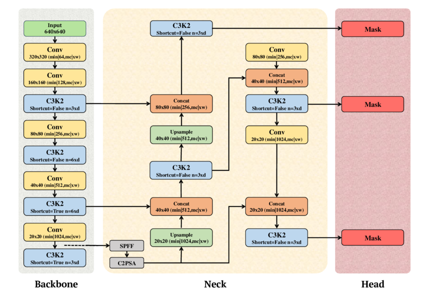
Fig. 1. Schematic diagram of YOLO11 showing the Backbone, Neck, and Head components (adapted from A. T. Khan and S. M. Jensen, LEAF-Net, Dec. 2024). 

Dataset 

Choosing the correct dataset was another fundamental decision in the YOLO Inference benchmark integration task, as it serves as the ground truth for our benchmark’s validity. We selected COCO 2017 (Common Objects in Context) because it was used to train YOLO models and remains the gold standard for object detection. With 80 object categories and over 1.5 million instances, we can ensure that the model won’t just memorize shapes but also truly understand spatial relationships and the varied hidden components in realistic images [7]. The model was not trained by the group; we used a subset of the COCO validation dataset and verified that it maintained its original accuracy.

However, distributing a large-scale dataset for an open benchmark such as MLPerf poses legal and compliance challenges, particularly regarding commercial distribution rights. While the COCO annotations are open, some images from sources are marked “Non-Commercial,” which means they are not compliant with commercial benchmarking. To address this, the Task Force developed a custom filtering pipeline to create a safe subset of the full COCO 2017 dataset. This ensures that the final dataset used by our partners is fully distributable and legally safe for both academia and industry, without compromising the benchmark’s statistical integrity. 

The MLPerf Subset 

Dataset	# of classes	# of validation images	Size
COCO Full	80	5000	~170 MB
COCO MLPerf	80	1525	~52 MB

Table 1: The COCO MLPerf subset shows the total number of safe images compared to the full dataset.

Loadgen integration

After creating the  COCO dataset, we had to ensure consistent accuracy scores in our YOLO LoadGen integration. MLCommons LoadGen (Load Generator) is a reusable C++ library with Python bindings that effectively and fairly measures the performance of ML inference systems by generating standardized query traffic patterns to ping the model across scenarios such as SingleStream, MultiStream, and Offline. The LoadGen API records all queries and responses for verification and summarizes whether performance latency constraints are met. While remaining model-agnostic and not specifically handling accuracy evaluation, the LoadGen API generates files needed for model-specific accuracy metric calculations [8].

Originally, the YOLO11 implementation generated a standard predictions.json file. While this format is sufficient for general COCO validation, it was incompatible with the COCO MLPerf Accuracy script for several reasons:

• Class mapping inconsistency: YOLO models traditionally use an 80-class index (0-79) derived from the COCO dataset. However, for the MLPerf accuracy evaluation, we wanted to use the 91-category COCO mapping, where class IDs are non-sequential.
• Coordinate normalization: The standard YOLO outputs are often absolute pixel coordinates or in the XYWH (standard x, y coordinates, width, height) format. For our accuracy evaluation, we wanted to use a specific serialized payload: a 7-element float array containing [index, y_min, x_min, y_max, x_max, score, class]. Crucially, these coordinates must be normalized (between 0.0 and 1.0) relative to the original image dimensions.
• Buffer serialization: Unlike a standard JSON dump, the MLPerf LoadGen requires results to be serialized into a byte buffer through the QuerySamplesComplete API.

Once we identified and resolved the issues above, we achieved matching mAP results to the Ultralytics reference using our YOLO LoadGen implementation. We got it to work with the following strategy:

• Class re-indexing: We implemented a robust mapping layer using the official COCO 80-to-91 conversion array. This ensures that every detection reported by YOLO is immediately translated into the category ID space recognized by the accuracy script.

Target ID = COCO_{80_to_91}[Model Class Index]

• Coordinate transformation: The Runner.enque logic was rewritten to handle image geometry dynamically. We first extracted the original height (H) and width (W) from the Ultralytics results object to perform a real-time normalization of the XYXY bounding box:

y_min = box[1] / H

x_min = box[0] / W

y_max = box[3] / H

x_max = box[2] / W

• LoadGen native serialization: We utilized the struct.pack(“7f”, …) method to create a binary payload. This payload is then passed directly into lg.QuerySampleResponse, allowing the MLPerf LoadGen to handle the logging in its native binary format. This change not only fixed the accuracy reporting but also reduced I/O overhead during performance runs by eliminating the need to write to an intermediate file.

By shifting this logic directly into the LoadGen runner, we achieved seamless integration, with mlperf_log_accuracy.json generated to the exact schema required by the accuracy-coco.py script. This ensures that mAP calculations are bit-accurate and directly comparable with other submissions in the MLPerf Inference leaderboard.

Performance evaluation 

For the edge suite, the following performance metrics are measured for the standard MLPerf scenarios: 

1. Offline, where the goal is to measure peak throughput (samples/sec) by processing the entire dataset as a single batch. In this benchmark scenario, LoadGen will send all queries to the System Under Test (SUT) at the start.
2. Single-Stream focuses on the absolute minimum latency for a single image – critical for real-time edge responses. LoadGen sends the queries to the SUT as soon as the previous one completes. The duration of this scenario is set to 1024 queries and 60 seconds.
3. Multi-Stream simulates multiple channels and measures the maximum number of concurrent streams the system under test can support. LoadGen sends queries to the SUT using the same method as Single-Stream, but the run duration is longer, at either 270,336 queries or 600 seconds.

As a single-stage detector with an optimized detection head, YOLO11 eliminates several post-processing and anchor-heavy computation stages present in RetinaNet, ultimately demonstrating a significant improvement in end-to-end inference 

Accuracy metrics 

While RetinaNet provided strong detection accuracy due to its focal loss formulation and multi-scale FPN backbone, YOLO11 achieves superior mAP while also delivering on latency [9]. Our implementation uses the mAP@50-95 standard, a metric that computes the average precision across ten Intersection over Union (IoU) thresholds (0.5-0.95). By doing so, we want to see that the model not only identifies the correct class but also localizes it with high pixel-level accuracy. We found this to be a challenging yet fair set of parameters for the YOLO11l model to maintain high throughput while ensuring that its bounding box predictions are nearly identical to the ground truth. 

We established two distinct target accuracy thresholds: yolo-95 and yolo-99. These represent 95% and 99% of the state-of-the-art reference score, respectively. The yolo-95 threshold serves as the “default” mode, allowing for submissions that prioritize system speed and throughput for standard production needs. In contrast, the yolo-99 threshold represents the “high accuracy” standard for mission-critical applications, requiring the model to converge almost perfectly to the reference accuracy. The mAP scores for the two modes are determined by taking the YOLO11l mAP score from Ultralytics and multiplying it by 0.95 and 0.99 for the default and high accuracy modes respectively. The table below shows a score of 53.4 for YOLO11l from Ultralytics, which translates to 0.534 * 0.95 for the yolo-95 version and 0.534 * 0.99 for the yolo-99 version. By offering these two tiers, the MLPerf benchmark allows hardware vendors to showcase different optimization profiles. 

Model variant	Parameters	mAP (COCO)	Ideal use case
YOLO11 nano	~2.6 M	39.5	Mobile/IoT edge
YOLO11 large	25.3 M	53.4	MLPerf Inference v6.0 choice
YOLO11 extra large	~59.6 M	54.7	High accuracy Cloud/Server

Table 2: Parameters and accuracy comparison of YOLO11 model variants.

Reference implementation 

The reference implementation for YOLO11 uses the official Ultralytics YOLO11 inference code. For readers interested in running the model in their own environment, we recommend following this MLCommons reference implementation, which includes the code and instructions for running the end-to-end benchmark, starting with the dataset and model downloads. 

Conclusion 

In summary, the transition from RetinaNet to YOLO11 marks a pivotal evolution in the MLPerf™ Inference benchmark, as the upgrade to a better model reflects industry trends. By adopting the YOLO11l variant, we are challenging hardware vendors to optimize for attention-augmented components like the C2PSA block. This shift ensures that our performance metrics are not just theoretical numbers, but actionable data points that translate directly to the efficiency and responsiveness of real-world AI use cases. 

Furthermore, the introduction of the yolo-95 and yolo-99 accuracy tiers provides a nuanced framework for AI infrastructure evaluation. It allows organizations to showcase the raw speed of aggressive quantization at the 95% threshold while maintaining a path for mission-critical, high-fidelity deployments at the 99% level. This benchmark will continue to serve as a positive step forward for the community, driving innovation and ensuring that the next generation of AI hardware is built to handle the complexity and scale of computer vision. MLCommons will continue working with domain experts and industry members to update the object detection models, ensuring that the MLPerf benchmark remains current and accurately reflects evolving industry trends.

Acknowledge

We would like to express our gratitude to the following individuals for their help and guidance during the development of this benchmark:

• Anandhu Sooraj (MLCommons)
• Arjun Suresh (MLCommons)
• Ashutosh Dhar (NVIDIA)
• Karl Pietri (MLCommons)
• Miro Hodak (AMD)
• Reilly Fairbanks (MLCommons)
• Scott Wasson (MLCommons)
• Zhihan Jiang (NVIDIA)

References

1. J. Redmon, S. Divvala, R. Girshick, and A. Farhadi, “You Only Look Once: Unified, Real-Time Object Detection,” arXiv preprint arXiv:1506.02640, Jun. 2015. [Online]. Available: https://arxiv.org/abs/1506.02640
2. Ultralytics, YOLO11 Model Documentation. [Online]. Available: https://docs.ultralytics.com/models/yolo11/
3. R. Girshick, “Rich feature hierarchies for accurate object detection and semantic segmentation,” arXiv preprint arXiv:1311.2524, Nov. 2013. [Online]. Available: https://arxiv.org/abs/1311.2524
4. S. Author, T. Author, and L. Author, “YOLOv1 to YOLOv11: A Comprehensive Survey of Real-Time Object Detection Innovations and Challenges,” arXiv, Aug. 2025. [Online]. Available: https://www.arxiv.org/pdf/2508.02067
5. M. Tan, R. Pang, and Q. V. Le, “EfficientDet: Scalable and Efficient Object Detection,” arXiv preprint arXiv:1911.09070, Nov. 2019. [Online]. Available: https://arxiv.org/abs/1911.09070
6. N. Carion et al., “End-to-End Object Detection with Transformers,” arXiv preprint arXiv:2005.12872, May 2020. [Online]. Available: https://arxiv.org/abs/2005.12872
7. T. Lin et al., “Microsoft COCO: Common Objects in Context,” arXiv preprint arXiv:1405.0312, May 2014. [Online]. Available: https://arxiv.org/abs/1405.0312
8. E. Hall et al., “MLPerf Inference Benchmark,” arXiv, Nov. 2019. [Online]. Available: https://arxiv.org/pdf/1911.02549
9. T.-Y. Lin et al., “Focal Loss for Dense Object Detection,” arXiv preprint arXiv:1708.02002, Aug. 2017. [Online]. Available: https://arxiv.org/abs/1708.02002
10. **A. T. Khan and S. M. Jensen, “The schematic diagram of YOLOv11 illustrating its three core components: Backbone, Neck, and Head,” inLEAF-Net: A Unified Framework for Leaf Extraction and Analysis in Multi-Crop Phenotyping Using YOLOv11, preprint, Dec. 2024. Fig. 5. [Online Image]. Available:https://www.researchgate.net/figure/The-schematic-diagram-of-YOLOv11-illustrating-its-three-core-components-Backbone-Neck_fig1_386467184