
Recommendation has long been part of MLPerf Training through the DLRM benchmark, which times how long a system takes to train a personalized recommendation model to a set quality target. The current version, DLRMv2 [1], is designed to recommend content based on user behavior and item features, using deep learning to capture the interactions between the two and produce more relevant suggestions on platforms such as e-commerce sites and streaming services. With recent advances in sequence modeling, including LLMs, production recommendation systems at hyperscale operators have shifted from compressing user behavior into a small set of aggregated dense features to representing each user’s recent interaction history as a per-event token sequence [2][3]. Models built this way keep improving as compute and parameters grow, while earlier feature-interaction designs flatten out. MLPerf has already brought this class into the inference suite with an HSTU-based benchmark [4], but the training suite still has no equivalent workload, leaving a fast-growing category of production training uncovered.
DLRMv4 fills that gap by replacing the feature-interaction stack with HSTU [2], a transducer that reads a user’s interaction history directly as a sequence, and it trains with a new dataset, Yambda-5B [5], a real multi-behavior collection of music listening activity, scaled to a production-class embedding footprint of 560 GB. Building on HSTU also keeps the training benchmark aligned with the inference benchmark that already represents this class of models. DLRMv4 will advance the training benchmark to more accurately reflect the state-of-the-art production DLRM workload, both in computational complexity, which now involves attention over long user histories, and in embedding table size, which requires sharding across multiple modern accelerators.
In the rest of this article, we walk through the new HSTU model architecture and the Yambda-5B dataset in more detail, explaining the design choices behind each, as well as the reference implementation, including its convergence behavior and measured system performance.
Model Architecture
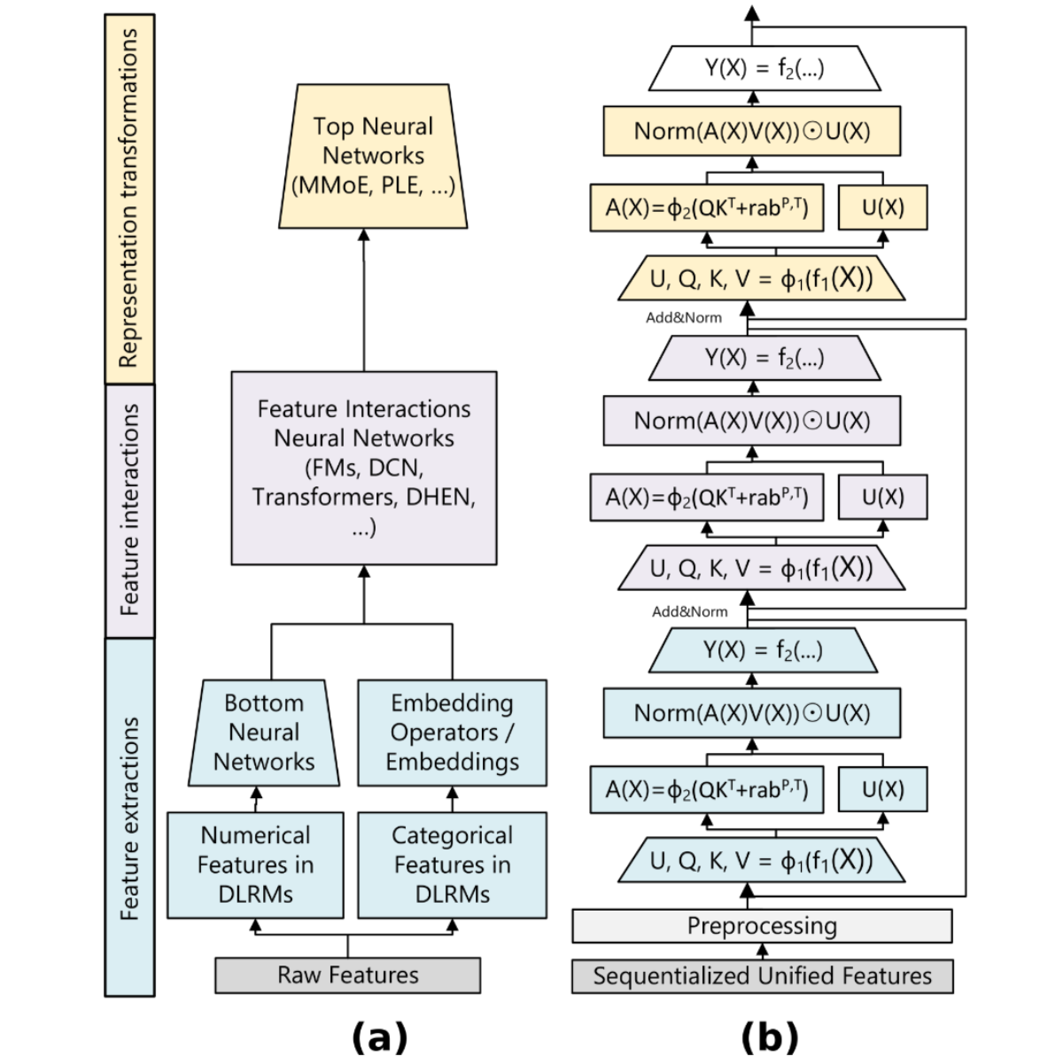
Figure 1: Traditional DLRM architecture(a) vs HSTU (b)
Figure 1 compares HSTU with the prior architectural pattern it replaces. Panel (a) shows the encode-then-interaction pipeline that has dominated production recommendation since DLRMv2 [1]. Inputs arrive in heterogeneous forms and are first lifted by a feature-extraction stage: bottom MLPs handle numerical features while embedding lookups handle categorical IDs. Their outputs are passed to a dedicated feature-interaction module, typically a cross network, a factorization machine, or a similar block, and finally to a task head that produces the prediction. The interaction module is where most modeling effort has gone, but it never sees the raw behavior stream. It works on hand-engineered, pre-aggregated inputs such as decayed counters, ratios, and pooled embeddings.
Panel (b) shows HSTU [2], which removes that division of labor. The heterogeneous feature space is first sequentialized into a unified time series: categorical and slowly varying features are merged into the user’s chronological history of items and actions, and the whole series is consumed end to end by a stack of identical transduction layers. Each layer folds together the three stages that a DLRM keeps separate. A single projection produces all the internal representations a layer needs; a pointwise attention step aggregates across the sequence using a bias derived from how far apart two events are in position and in time; and a gated transformation lets the attention-pooled features interact directly, taking over the role of both the explicit cross network and the feed-forward block. Because the same block simply repeats, the design surface collapses to three scaling axes, depth, width, and sequence length, that govern the entire backbone. The HSTU work quantifies the payoff as a power-law relationship between compute and quality that holds across three orders of magnitude, in a regime where the encode-then-interaction baseline flattens out.
It helps to follow a single training example. Suppose the model is scoring one candidate item for a given user on a content platform. The user’s interaction history is assembled as an interleaved stream of past items and the actions taken on them, drawn from several behavior types such as genuine engagements, explicit approvals, and skips, and truncated to a fixed budget of a few thousand events. Each event becomes one token that carries what the item was, what the user did with it, and when that happened, so a negative signal such as a skip stays in the sequence as a first-class event instead of being averaged away into a counter. Slowly-varying context, including the user’s identity and precomputed cross features, is compressed into a handful of prefix tokens at the head of the same series. The candidate being scored is appended at the end, which lets the model compare it against the history in a single pass rather than through a separate target-aware pooling step. The stack then processes this one sequence, and the representation at the candidate position feeds a small head that emits the engagement prediction.
Handling history, context, and candidate jointly in one causal block is what makes HSTU both production-relevant and a demanding systems workload, and it is the same configuration that underpins the MLPerf DLRMv3 inference benchmark [4].
Dataset
DLRMv4 trains on Yambda-5B [5], the largest open recommendation dataset with multi-behavior real-user interactions, released publicly by Yandex Music. The benchmark uses the full 5B-event variant, whose headline properties are summarized below.
| Property | Value |
| Source | Yandex Music public release |
| Interactions | ~4.79B |
| Users | 1M |
| Items | 9.39M |
| Behavior types | 5 (listen, like, dislike, unlike, undislike) |
| Raw size | ~38 GB (for the Yambda-5b variant) |
| Per-event bytes | ~20 |
Table 1: Yambda-5b Dataset Properties
Compared with the previous DLRMv2 benchmark’s Criteo 1TB dataset [1], Yambda is a better fit for an HSTU-style model because it provides what such a model requires: a real per-user timeline. Every interaction is recorded with the user who made it, the item it touched, the action type, and when it happened, so each user’s history can be reconstructed in chronological order and handed to the transducer as a sequence. With roughly 4.79B interactions, the dataset is large enough to keep a full-scale training run under sustained load.
| Criterion | Criteo 1TB (DLRMv2) | Yambda-5B (DLRMv4) |
| Real data | Yes | Yes |
| Interaction volume | 4.2B rows | 4.79B rows |
| Per-user history | No (flat features only) | Yes (multi-behavior pools) |
| On-disk size (raw data) | ~4 TB(denormalized) | ~38 GB (normalized) |
| Embedding Table Size | ~100 GB | ~560 GB (after adding cross-feature tables) |
| HSTU-aligned | No (no sequence axis) | Yes |
Table 2: Comparison between Yambda-5b and Criteo 1TB(DLRMv2) datasets
We extend Yambda’s four native sparse features (item, artist, album, uid) with cross-product hashed tables. Cross features are standard practice in industrial recommenders, where explicitly representing feature conjunctions such as (user, artist) or (item, hour-of-day) has long been used to boost ranking quality [7][8], and recent work suggests the benefit scales continuously with the memory allocated to them [9]. Including them keeps the benchmark representative of production models and brings the embedding table footprint to approximately 560 GiB, with 512 embedding dimension and fp32 embedding precision:
| Table | Category | Cardinality | Size(512 embedding dimension, fp32) |
| item | native | 9.39M | 19.2 GB |
| artist | native | 1.29M | 2.6 GB |
| album | native | 3.37M | 6.9 GB |
| uid | native | 1M | 2.0 GB |
| user × artist | cross feature | 100M | 204.8 GB |
| user × album | cross feature | 40M | 81.9 GB |
| user × hour | cross feature | 24M | 49.2 GB |
| item × hour | cross feature | 40M | 81.9 GB |
| artist × hour | cross feature | 32M | 65.5 GB |
| user × is_organic | cross feature | 2M | 4.1 GB |
| user × artist × hour | cross feature | 40M | 81.9 GB |
| Total | ~560 GB |
Table 3: Feature Expansion of Yambda-5b via Cross-product Feature Tables
Real recommendation traffic is heavily skewed: a small number of items account for a large share of all interactions, and a benchmark is only representative if its data behaves the same way. To confirm this holds, we analyzed the Yambda-5B dataset, measuring how often each individual row of the item, artist, and album embedding tables was read across a sample of roughly 205,000 real interaction events. All three follow the classic Zipf pattern closely (Table ), with popularity concentrated in a small head of the catalog. The skew the hardware sees is sharper still, because each event is read back through many overlapping user histories: the top 1% of touched rows absorb 52–68% of all embedding lookups, and the top 10% absorb over 90%. That is precisely the pressure that makes embedding sharding a real problem at this scale.
| Table | Zipf exponent | Fit quality(R^2) | Share of total interactions: Top 1% of rows | Share of total interactions: Top 10% of rows |
| item | 0.53 | 0.99 | 16% | 50% |
| album | 0.6 | 0.98 | 18% | 54% |
| artist | 0.83 | 0.96 | 24% | 67% |
Table 4: Popularity skew of the Yambda-5B native id tables, measured on sampled training data. Zipf exponent is the slope of the popularity-rank curve. Fit quality (R^2) measures how closely the curve follows a straight Zipf line.
Reference Implementation
The reference implementation extends Meta’s open-source HSTU implementation [6], the same codebase behind the DLRMv3 inference benchmark, and integrates it with the Yambda-5B dataset: a preprocessing and streaming pipeline turns the raw multi-behavior event log into per-user interaction sequences the HSTU stack can consume, and a set of cross-feature tables built on the dataset’s native vocabularies brings the embedding footprint up to production scale.
HSTU Hyperparameters
The reference model is a 3-layer HSTU stack with 4 attention heads, a model dimension of 512, attention linear and query/key dimensions of 128, and a max sequence length of 4,096. Training runs in bf16 mixed precision, with attention computed by a fused jagged-attention Triton kernel. We optimize the dense parameters and embedding tables separately, using Adam for the dense parameters and row-wise Adagrad for the sparse embedding tables. The learning rate warms up to a target that scales with the global batch size, compensating for the fact that larger batches need more samples to converge. The main hyperparameters are listed in the table below (we defer the discussion on the choice of learning rates to the Convergence Evaluation section):
| Hyperparameter | Value |
| HSTU attention layers | 3 |
| Max sequence length | 4096 |
| Number of attention heads | 4 |
| Model(transducer) dimension | 512 |
| Per-head dimension | 128 |
| Precision | bf16(mixed) |
| Dense optimizer | Adam |
| Sparse optimizer | RowWiseAdagrad |
| Learning Rate Warmup | 24000 steps |
| Target Learning Rate by Global Batch Size | 8k: 1e-6 16k: 2e-6 32k: 4e-6 |
| Embedding table dimension | 512 |
Table 5: Main HSTU Hyperparameters Used by Reference Implementation
Benchmark Computation Cost Analysis
In this section, we perform some computation cost analysis based on the corresponding model and training hyperparameters. Below we define the symbols and corresponding values used in the cost analysis:
| Symbol | Value | Meaning |
| B | 1024 | Per-GPU batch size |
| L | 3 | Number of HSTU layers in the transduction stack |
| h | 4 | Attention heads per layer |
| d_qk | 128 | Per-head Q/K dimension |
| d_v | 128 | Per-head V/U dimension |
| D | 512 | Model (transducer) dimension |
| S | 4096 | Max sequence length |
Table 6: Cost Analysis Symbols
Below it shows the total computation cost and the breakdown of each component
| Component | FWD+BWD cost expression | Cost per GPU step (TFLOPS) |
| UVQK GEMMs | B · L · 3 · 2 · S · D · (2·d_qk + 2·d_v) · h | 79.16 |
| Output projection GEMMs | B · L · 3 · 2 · S · (3 · h · d_v) · D | 59.37 |
| HSTU attention(causal) | B · L · 3.5 · 2 · (S² / 2) · h · (d_qk + d_v) | 184.72 TFLOPs |
| Total | 323.26 TFLOPs |
Table 7: Computation Cost Analysis Breakdown by HSTU Component
Weight GEMMs are counted at a multiple of 3 for forward-plus-backward, since the backward produces both an input gradient and a weight gradient. Attention is counted at a multiple of 3.5, because its backward produces dQ, dK, and dV in roughly five GEMMs against the forward’s two. Attention is additionally counted at a multiple of 1/2 for causality: HSTU attention is causal, and the kernels evaluate only the lower triangle.
Convergence Evaluation
| Examples to convergence (AUC 0.75) | Training time to convergence (AUC 0.75) | |
| LR=1e-6 | 68.8M | 125.4 minutes |
| LR=1e-7 | 217.6M | 396.3 minutes |
Table 8: Convergence Comparison between Different Learning Rates for 8k Batch Size
We first evaluated convergence behavior under different learning rates to choose a suitable range for the benchmark. We generally found that while lower learning rates provide more stable convergence trends across multiple runs, they also could require orders of magnitude more examples to converge to the same AUC target. Table 9 compares 1e-6 and 1e-7 learning rates with the same 8k global batch size. The result shows that for an 8k global batch size, if we lower the learning rate from 1e-6 to 1e-7, it will take 3 times the training examples to converge to the same 0.75 AUC target, which also means roughly 3 times more training time with the same training throughput(125 minutes to 396 minutes). To balance convergence time in an efficient training performance evaluation benchmark with training stability, we choose 1e-6 as the target learning rate for an 8k batch size and use learning-rate warmup to reduce variability across multiple runs with different seeds. Without learning-rate warmup, a high learning rate like 1e-6 could cause large variance in training examples and thus increase the time to reach convergence across runs with the same training performance, defeating the purpose of the benchmark. (For real submission, we would allow some degree of flexibility regarding the choice of target learning rate, e.g. [0.5*LR, 1.5*LR] where LR is the reference learning rate used to generate RCP convergence curves below, in order to reduce the submitter effort when dealing with the different convergence behaviors caused by software/hardware differences against the ones we used to generate RCP.)
We then ran convergence tests with different batch sizes to determine how much data the model needs to reach the quality target, and how reliably it gets there on MI350 GPUs. To balance meaningful training time for evaluating performance versus stability across runs, we set AUC 0.75 on the held-out data as the convergence target, and define convergence as the first evaluation that crosses it. The sweep is 3 global batch sizes × 20 seeds (60 runs), where each run at a given batch size uses a different random-initialization seed, with eval_accuracy recorded every 0.1% of the training data. (For real submission, we would use a formula to skip the early evaluation passes to save time.)
| Global batch size | Number of GPUs | Samples to converge to AUC 0.75(min/mean/max) | Wall-clock to AUC 0.75 (min/mean/max) | CV |
| 8192 | 8 | 61.9M / 69.3M / 80.3M | 2h22m / 2h39m / 2h59m | 5.6% |
| 16384 | 16 | 78.0M / 87.7M / 100.9M | 1h39m / 1h52m / 2h12m | 7.2% |
| 32768 | 32 | 98.6M / 113.0M / 128.5M | 1h17m / 1h23m / 1h36m | 6.7% |
Table 9: For each batch size, the table reports the GPU count it ran on (per-rank batch 1024), how many samples the 20 seeds needed to reach the target, the wall-clock to get there, and the spread across seeds as a coefficient of variation.
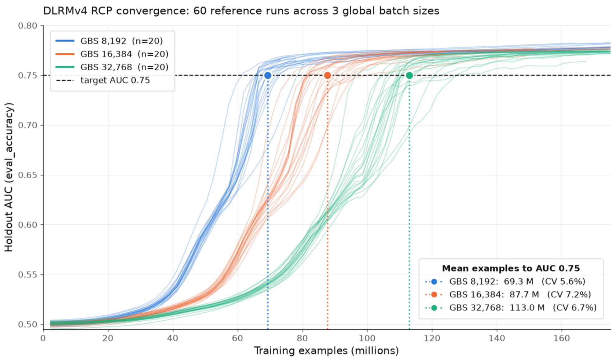
Figure 2: Convergence Curves for the RCP Runs of Different Global Batch Sizes 8k/16k/32k
The runs all converge to AUC 0.75. CV is the sample standard deviation of the 20 per-seed sample counts divided by their mean, and it stays between 5.6% and 7.2%, which is tight enough that a single run represents its batch size despite different initialization.
To reduce the sample penalty for larger batch sizes, we scale the learning rate linearly with batch size, and the resulting sample penalty for larger batches is reasonable. Quadrupling the global batch from 8,192 to 32,768 costs only 1.63× the samples (69.3M to 113.0M mean), with the target learning rate scaled linearly and everything else fixed. Convergence still lands within the first 3–5% of one epoch over the 2.29B-sample training set. Figure 2 illustrates the convergence curves for the RCP runs generated for different batch sizes.
Conclusion
DLRMv4 brings MLPerf Training in line with how production recommendation systems are actually built today: sequence models over real user histories, attention over thousands of events, and embedding tables measured in hundreds of gigabytes. By establishing a common model, dataset, quality target, and evaluation procedure, MLCommons gives the industry a practical way to measure progress on this fast-growing class of workloads. The benchmark specification and reference implementation are available on GitHub.
We thank the DLRMv4 task force for coming together to bring production-scale recommendation to MLPerf Training.
About MLCommons
MLCommons is the world’s leader in AI benchmarking. An open engineering consortium supported by over 125 members and affiliates, MLCommons has a proven record of bringing together academia, industry, and civil society to measure and improve AI. MLCommons began with the MLPerf benchmarks in 2018, which quickly grew into a set of industry metrics for measuring machine learning performance and promoting transparency in machine learning techniques. Since then, MLCommons has continued to use collective engineering to build the benchmarks and metrics required for better AI – ultimately helping to evaluate and improve the accuracy, safety, speed, and efficiency of AI technologies.
For additional information on MLCommons and details on becoming a member, please visit MLCommons.org or email [email protected].
Reference
[1] DLRM-DCNv2, MLPerf Training recommendation benchmark. https://github.com/mlcommons/training/tree/master/recommendation_v2/torchrec_dlrm
[2] Actions Speak Louder than Words: Trillion-Parameter Sequential Transducers for Generative Recommendations. https://arxiv.org/abs/2402.17152
[3] OneTrans: Unified Feature Interaction and Sequence Modeling with One Transformer in Industrial Recommender. https://arxiv.org/abs/2510.26104
[4] DLRMv3: Generative recommendation benchmark in MLPerf Inference. https://mlcommons.org/2026/02/dlrmv3-inference-meta/
[5] Yambda-5B — A Large-Scale Multi-modal Dataset for Ranking and Retrieval. https://arxiv.org/abs/2505.22238
[6] Generative Recommenders, Meta. https://github.com/meta-recsys/generative-recommenders
[7] Wide & Deep Learning for Recommender Systems. https://arxiv.org/abs/1606.07792
[8] DCN V2: Improved Deep & Cross Network and Practical Lessons for Web-scale Learning to Rank Systems. https://arxiv.org/abs/2008.13535
[9] MemoNet: Memorizing All Cross Features’ Representations Efficiently via Multi-Hash Codebook Network for CTR Prediction. https://arxiv.org/abs/2211.01334