Introduction
Generative AI models have been getting a lot of attention in recent years, and image generation models in particular have piqued interest among researchers, developers, and the public. The widespread adoption of image generation motivated us to add a new benchmark to the v4.0 round of MLPerf Inference using the Stable Diffusion XL model. This blog describes the complexities involved in benchmark construction such as model and dataset selection, with a particular focus on accuracy metrics. We believe these design choices address most of the critical deployment decisions faced by practitioners while delivering important performance insights to customers.
The evolution of image generation models can be grouped into three architectural eras: autoencoders, generative adversarial networks (GANs), and diffusion models.
Autoencoders are characterized by an encoder-decoder architecture where the encoder compresses a high-dimensional image into a low-dimensional representation in a latent space. When the latent space is mapped into a probability distribution, this network turns into a generative model where we sample latent representations and project them to image space using a decoder. This class of models is called variational autoencoders (VAEs.) VAEs set a benchmark in terms of image quality and ease of training, and this type of model is still being used as a key component in diffusion models.
GANs, first published in 2014, employ the novel idea of dueling networks: a generator and a discriminator. The generator is trained to take in Gaussian noise and produce realistic images, and the discriminator is trained to identify whether the generated image is real or fake. Once trained, the generator can be used as a stand-alone network to produce realistic images. One key drawback of GANs is that they tend to be challenging to train; it can be difficult to get them to converge, and sometimes they experience mode collapse where the GAN converges on a very limited set of outputs, limiting their expressiveness.
Diffusion models, the latest development in generative image models, offer the potential to generate a broader range of images with higher fidelity than GANs. Inspired by physics, the idea behind diffusion models is to learn the structure of the dataset by modeling the way data diffuses through the latent space. Diffusion models are trained to add and remove small amounts of Gaussian noise in repeated steps. During inference or generation, the model undergoes a reverse diffusion process where it considers a text prompt, starts with a randomly generated noisy image, and gradually works to denoise it until a predefined number of steps is reached.
Many diffusion models with varying approaches, such as Dall-E, Midjourney, and Imagen, have shown great potential in generating realistic images in recent years. One of the most important breakthroughs for diffusion models was the introduction of latent diffusion models (LDMs) in December 2021. The key differentiator in this family of models is that the entire diffusion process happens in latent space instead of pixel space. This is done using a VAE encoder which compresses the images into a low dimensional latent vector, performs the diffusion process with a U-Net backbone, and then finally uses a VAE decoder to project the latent back to the pixel spaces. This arrangement reduces the cost of training and inference substantially because the expensive denoising process in the latent space and therefore involves fewer parameters.
With increasing interest and adoption of LDMs and text-to-image models in general, MLCommons believed that a fair and robust benchmark in this domain for the deep learning community was needed. With this goal in mind, the MLPerf Inference working group formed a special task force in September 2023 to explore, define, and create a text-to-image-diffusion benchmark.
Choosing the model and its scheduler
The task force looked for candidate models that were openly available with compatible licenses, were popular in use, and produced state-of-the-art results. The candidates considered included Stable Diffusion (SD) 1.5 and 2.1 and Stable Diffusion XL (SDXL) 1.0. After deliberation, the task force chose SDXL 1.0 for the benchmark, and was subsequently introduced in the MLPerf Inference v4.0 benchmark round.
Stable Diffusion XL 1.0 is a diffusion model developed by Stability AI. By September 2023, it was the latest and largest open source text-to-image model that generated high-resolution (1024×1024) images with default settings. In comparison, SD 2.1 generated 768×768 images, and SD 1.5 generated 512×512 images. Higher resolution matters because it allows for greater detail and clarity in the generated images, making them more visually appealing and useful for various applications.
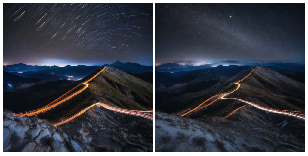
SDXL has two variants: SDXL-base (roughly 3.5 billion parameters) and SDXL-refiner (about 6.6 billion parameters). Both are significantly larger and more challenging than SD v2.1 (860 million parameters) and SD v1.5 (983 million parameters), adding a quantitative novelty to MLPerf Inference benchmark. The refiner model improves the fine-grained details in the generated images, as illustrated in Figure 1. However, this modest qualitative improvement comes at the cost of nearly double the parameters and compute requirements. Overall, we believe SDXL-base is a good compromise between practicality and pushing the limits of our machine-learning capabilities.
Figure 1: Left is output from SDXL-base, right is output from SDXL-refiner. Note the slight improvement in the shadowed skin texture on the neck in the right image compared to the left. Image courtesy: https://www.reddit.com/r/StableDiffusion/comments/15amidh/do_we_really_need_the_refiner_for_sdxl/
As depicted in Figure 2, SDXL has two dedicated networks, CLIP1 and CLIP2, that encode text prompt tokens into an embedding space. Using two networks better captures semantic information compared to the use of a single CLIP network in other diffusion models. SDXL also leverages a larger U-Net backbone than SD. The scheduler and the U-Net together denoise the image in latent space iteratively. The VAE decoder then recovers the image latent to a 1024×1024 RGB image output at the final stage.
Figure 2: Components of the text-to-image SDXL base pipeline
Schedulers are the algorithms that run multiple times iteratively to create a clean image from a completely random noisy image. The choice of scheduler determines the exact algorithm used to obtain a less-noisy latent. Some of the popular schedulers used for Stable Diffusion are DDIM, DDPM, and EulerDiscrete. Many scheduler algorithms involve a trade-off between denoising speed and quality, and each one works best with a particular number of steps. The speed of denoising mostly depends on the number of steps needed to reach a high-quality image.
The task force chose EulerDiscrete because it is one of the fastest schedulers available and has been widely adopted by users. From a qualitative standpoint, EulerDiscrete typically can produce clear images with almost no color artifacts in 20-30 steps, while DDIM requires around 50 steps. Quantitatively, the task force experimented with Hugging Face diffusers and showed that EulerDiscrete with 20-30 steps produced FID scores (a common quality metric that we discuss later) similar to those of DDIM scheduler with 50 steps.
Choosing the dataset
The choice of dataset is pivotal for the evaluation of an image-generation model. Each image in the dataset should be paired with a descriptive prompt that effectively communicates the visual content and context. This pairing enables the model to be assessed on its ability to generate images that are not only visually appealing but also contextually appropriate. The dataset should be diverse enough to cover various scenarios and object types in order to ensure the model’s performance is tested across different contexts.
The task force determined that the Common Objects in Context (COCO) dataset was an excellent match for this task. This dataset is recognized in the ML community for its diversity and for the richness of context in its image-caption pairs. A random subset of 5,000 prompt-image pairs were selected for the benchmark. This subset size is sufficient to ensure broad coverage and variety while being manageable for computational cost. Cross-validation tests verified that this random selection does not significantly alter the quality metrics. Additionally, COCO’s widespread use for similar tasks in the research community ensures relevance and comparability with the overall field.
Downloading the COCO images is not necessary for the benchmark evaluation. Instead, the FID score can be computed using pre-calculated statistics from the COCO dataset. Similarly, when using the CLIP score, the focus is on how well the output images correlate with the input prompts rather than with the ground-truth images.
Negative prompts are an extremely common guiding mechanism for image generation. Users can specify what they want to exclude from generation and also guide the output image away from undesired stylistic elements (e.g., avoiding cartoonish styles or unwanted elements like cars or buildings). Unfortunately, the task force could not find a suitable dataset with negative prompts. Since this is a crucial feature to the end user that also impacts performance, several prompts were analyzed, and a single common negative prompt was selected for all samples. Prompt “normal quality, low quality, worst quality, low res, blurry, nsfw, nude” generated the best results while adding additional content moderation safeguards beyond what a filtered training dataset provides and was therefore used in the benchmark.
Challenges of measuring accuracy
Evaluating generative AI models designed for image generation presents several unique challenges that we had to resolve to construct a representative and effective benchmark. A primary issue is the absence of a definitive “ground truth,” since the success of these models often depends on how well the generated images meet varying user expectations rather than adhering to an objective standard. Furthermore, the stochastic nature of these models means that output depends on the initial noise that seeds the model. Although the initial noise input can be controlled, as seen in Figures 3 and 4, the model pipeline remains sensitive to changes in hardware and software configurations. Minor adjustments to the pipeline (such as the use of quantization) can lead to wildly varying outputs. This variability rules out the use of error-based metrics such as mean squared error (MSE), root mean squared error (RMSE), or peak signal-to-noise ratio (PSNR), while also challenging the applicability of structural similarity index measure (SSIM)-based methods.

Figure 3: Two images created from the same prompt showcasing different optimization techniques. The image on the left was generated by an FP16 model, while the image on the right comes from an FP16+INT8 model featuring deep cache.

Figure 4: Visualization of the absolute error on each pixel when FP8 output from Intel Gaudi is compared to FP32 reference. The prompt was “some meat and vegetables are arranged on a white plate.”
In response to these challenges, the community has developed metrics to assess image-generating models quantitatively. The Fréchet inception distance (FID) measures the similarity between two sets of images (generated and real) by computing the Fréchet distance between two Gaussians fitted to feature vectors in an embedded space, typically derived from a pretrained inception network. However, the FID score alone is insufficient since it does not assess whether images accurately respond to the given prompts. So, the contrastive language-image pre-training (CLIP) score was chosen as an additional accuracy metric to evaluate the semantic relevance of the generated images to their textual descriptions. Since it is possible to optimize for one of these two metrics at the expense of the other, we explicitly require that both FID and CLIP scores be used in conjunction to ensure balanced optimization.
While these metrics can gauge certain aspects of the accuracy or quality of an image generation model, they have some shortcomings. Both metrics rely on pre-trained neural networks and can be sensitive to the choice of feature space and vulnerable to adversarial attacks. Also, they may not always correlate with human judgment of image quality. Moreover, FID requires a large sample of images to measure the distribution of a generated image dataset representatively, which can increase the cost and complexity of evaluation cycles. We acknowledge these limitations and are open to updating the benchmark in response to advances in this field.
Determining the accuracy threshold
Even though the U-Net latent noise input is fixed and the randomness is suppressed in our benchmark pipeline, different hardware and software can still produce varied outputs. To determine a reasonable accuracy threshold, the task force obtained the mean FP32 precision FID and CLIP scores on accelerators from multiple vendors for the 5,000-sample evaluation dataset. A ±2% variation limit for FID and ±0.2% variation limit for CLIP was set around this mean. FID was found to be more sensitive to hardware variation, hence the larger range. In this benchmark, a valid submission needs to achieve an FID score within the range of [23.01085758, 23.95007626] and CLIP scores within [31.68631873, 31.81331801].
Measuring performance
Figure 5: Generated images using SDXL with EulerDiscrete scheduler with 50 denoising steps (left) and 20 steps (right). There is a slight difference observed between 50 and 20 steps but no significant noise.
The run time of this particular benchmark depends on the number of denoising steps and the size of the validation set. An example can be seen in Figure 5. The task force conducted experiments to determine the optimum parameters that minimize the run time for performance and accuracy runs while maintaining the quality of generated images. As a result, 20 denoising steps and 5000 validation samples were chosen.
Robustness of the benchmark
Output reproducibility
SDXL starts the image generation with a latent space filled with random numbers from the standard normal distribution. In every following denoising step, a new image with less noise in the latent space is generated. In most applications, the initial latent state is defined by user-specified seed value for the random number generator. This arrangement allows for regenerating the same image later with more denoising steps and/or with different sampler settings.
The StableDiffusionXLPipeline used in our reference implementation relies on torch.randn which does not guarantee determinism across PyTorch releases and between different accelerators. MLPerf Inference rules restrict non-determinism, but submitters are free to use any framework for their submission. To ensure determinism, the task force decided to generate latent representations and provide them along with the reference implementation. Images from different accelerators with such a constant latent can be seen in Figure 6. Such a configuration helps to verify whether a submission maintains the model equivalence rule. This setup also enables the tightening of the FID and CLIP accuracy thresholds.
Qualcomm Cloud AI 100 submission | NVIDIA H100 submission |
Intel Gaudi 2 submission | HuggingFace fp32 reference |
Figure 6: Similar images are generated from four different accelerators thanks to setting a constant latent in the benchmark.
Compliance check
As noted earlier, FID and CLIP have limited capability in capturing the aesthetic assessment of generated images. Furthermore, the restricted non-determinism ensures the generated images from each submission are expected to be visually similar to the reference images generated from pytorch fp32 reference implementation. The task force therefore chose to add a human compliance check to the submission and review process for SDXL.
The task force decided to include a check that targets 10 image indices chosen using a random seed generator. Submitters are required to include the 10 images generated for these prompts along with their submissions. These images are inspected by submitters during the review stage of the results submission process. Any image determined to be a pure-noise image, such as a white noise image, or an image that presents a completely different semantic information than its text prompt will disqualify the corresponding submission. After successfully passing this human inspection, these images are removed from each submission before its publication.
Conclusion
In this blog post, we described the new SDXL benchmark introduced in the v4.0 round of MLPerf Inference, including the complexities involved in the choices of model and dataset. In particular, the current accuracy metrics for image comparisons have notable limitations, so we undertook several measures to ensure a robust benchmark. We believe these design choices capture the real challenges faced by practitioners and accurately and fairly represent performance for customers looking at adopting image generation.
Additional details about the MLPerf Inference Stable Diffusion benchmark and reference implementation can be found here.

